What do we do with the Earth's gravity and magnetic fields?
A basic statement for non-professionals
The primary goal of studying gravity and magnetic data is to provide a better understanding of the subsurface geology of the Earth. Gravity and magnetic measurements are both non-destructive remote sensing methods that are relatively cheap, and are used to determine information about the subsurface that is useful especially in exploration for oil and gas and mineral deposits.
 Gravity data provide information about densities of rocks underground. Because there is a wide range in density among rock types, geologists can make inferences about the distribution of strata that may be favorable for trapping oil and gas. For example, limestone, which is mostly the mineral calcite (calcium carbonate), has a relatively high density, sometimes as much as 2.8 grams per cubic centimeter, compared with some porous sandstones, which may have a density of 2.4. Pure rock salt has a very low density, about 2.15. Careful measurements of gravity can permit the interpretation of density (and therefore rock) distribution in the subsurface. Identifying a salt dome (a vertical column of salt that rises from great depth) will help locate many possible oil and gas traps.
Additional uses for accelerometers
 The magnetic field of the Earth is probably generated by electrical currents in the liquid outer core. Effectively, it is reasonable to think of the field as like that of a bar magnet at the earth's core, as shown in the picture on the left. It affects magnetic minerals that are distributed in many rocks in the crust, so that the rocks have a component of magnetization. For many purposes this is approximately proportional to the distribution of one mineral, magnetite (iron oxide), which is by far the most common magnetic mineral in the earth's crust. We can therefore determine the distribution of some rock types that are usually magnetite-rich. Most sedimentary rocks contain little magnetite, so generally we are "looking at" igneous and metamorphic rocks. Because of the nature of magnetic fields, geophysicists can determine the distance to the magnetite-rich rocks, which in turn suggests how thick (and how prospective) the overlying sedimentary rocks are. In the case of mineral exploration, such analysis can help pinpoint the locations of ore bodies.
If you have questions about the use of gravity and magnetic data for exploration, please feel free to contact . He'll try to answer!

Gravity and Magnetics Primer for Geoscientists

For a more thorough treatment, you are referred to any good geophysics textbook, such as Nettleton's Gravity and Magnetics in Oil Prospecting (McGraw-Hill, 1976).
Magnetic maps in the Former Soviet Union section illustrate some of the basic concepts of magnetic interpretation. In addition, you may be interested in Integrated Geophysics Corporation's Glossary of Terms. Through the courtesy of IGC, this Glossary was modified by IGC and others for inclusion in the AAPG book, Gravity and Magnetics Exploration Case Histories.
This section has benefitted from the comments of David Chapin, who is however in no way responsible for any errors of omission or commission!
Regional tectonic features expressed in the gravity map of the U.S.
Note: The official units for gravity and magnetic measurements are milligals (mGals) and nanoTesla (nT). In some reports and maps you may enounter gammas (1 gamma= 1 nanoTesla) or the abbreviation mgal. Also, some older gravity maps may be contoured in "gravity units." One gravity unit (g.u.) = 0.1 mGal. If you encounter (as I did in the Soviet Union work) milli-Oersteds, I can save you some work by letting you know that 1 milli-Oersted = 100 gamma = 100 nT.
After you wade through all these words, try the Grav-Mag Quiz at the bottom of the page!
Two qualities of potential-field data which are important to both
quantitative and qualitative interpretation are amplitude and frequency.
Amplitude, or intensity, refers to the value of a gravity or magnetic anomaly in milligals or gammas. In hydrocarbon exploration, gravity and magnetic anomalies are typically measured to 0.01 milligal and 0.01 gamma (nT), respectively, or better than one part in 5,000,000 of the earth's magnetic field, and even better than that for gravity. This instrument accuracy is attainable, but for most practical purposes in exploration surveys, realistic accuracies are on the order of 0.1-0.2 milligal and 0.5-1.0 gamma (nT). In general, the  value is proportional to the density or magnetic susceptibility contrast in the rocks beneath the sensor. (Susceptibility is a measure of the ease with which a material can be magnetized. Geologically, it can be thought of as a measure of magnetite content, although there are a few other minerals that contribute to bulk rock magnetization under special circumstances.) Again generally, gravity highs indicate the presence of relatively dense rocks, and magnetic highs are caused by rocks with abundant magnetite in them. Gravity highs might come from dense basalts or dense dolomites, but only the former are also magnetic. Thus specific lithologies may be implied, but statements about lithology in the subsurface are usually interpretations.
Sometimes the data are nearly inescapable in their implication of certain rock types (especially when diverse data are interpreted synergistically), but more often several alternatives are possible and should be constrained as much as possible with other information. Very high intensity anomalies (more than 50 milligals or more than 200 gammas) typify major rock type changes, usually (but not always) in basement rocks. 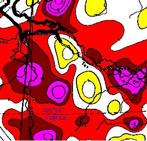 Thus, the magnetic map to the left, of the Zapolyarnoye area of West Siberia, with a contour interval of 100 nT, shows lithologic changes first and foremost. The intrabasement lithologic boundaries can be further interpreted, in this case as rift faults bounding basalt-filled grabens (magnetic highs) and horsts (magnetic lows) that contain drape anticlinal structures trapping huge gas fields. This interpretation is critically dependent on knowledge of the tectonic and geologic setting of the area.View a model through this horst.
Such changes are commonly clearer in magnetic data, reflecting the fact that magnetite content varies much more in basement rocks than does density. In fact, susceptibilities may vary by several orders of magnitude, while densities in the crust typically span only relatively small percentage changes (e.g., from perhaps 1.8 g/cc for porous diatomites to 3.3 g/cc for basalts and ultramafics. Within the basement, densities between 2.6 and 3.0 g/cc reflect a wide variety of igneous and metamorphic rock types.). Structural features, such as folds and faults, usually cause much smaller anomalies (Fig. 1). The observed anomaly is of course the result of both structural and lithologic effects; if a small anomaly caused by a large structure is superimposed upon a large anomaly caused by a lithologic contrast, the two features may be inseparable. Zones of lithologic contrast are often loci of structural disturbance.
Frequency is a measure of how narrow or broad anomalies are, and is a quantity which is mathematically proportional to the depth to sources. High-frequency, narrow anomalies come from sources that are relatively shallow, and broad, low-frequency anomalies are caused by contrasts at greater depths (Fig. 2). This quality of these data is irrespective of intensity; that is, a magnetic high that is very broad almost certainly comes from great depth. It is a mistake to equate magnetic highs with topographic or structural highs, just as magnetic highs should not necessarily be expected to coincide with gravity highs.
Because magnetic anomalies come from contrasts between relatively few rock types, quantitative analysis such as computing a depth to source is appropriate (if specifications of the data acquisition are known; in some data sets, such necessary parameters as magnetometer altitude may not be known). Gravity anomalies, as mentioned above, are caused by contrasts in all parts of the rock section and can therefore be misleading. It is possible for relatively shallow sources to be distributed in a way that produces a broad gravity anomaly which would be expected to come from deep bodies of rock. Computer modeling is appropriate for both gravity and magnetic data analysis. See Gibson's abstract on West Siberia for an example of a magnetic model.
Regional tectonic features expressed in the gravity map of the U.S.
by Dick Gibson
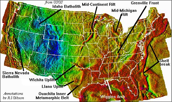 This discussion is in reference to an image of the complete Bouguer gravity map of the United States, provided by the USGS (annotations by Gibson). Note that some of this information is interpretive, and many details have been ignored in this general statement. And as with any geoscience data set, the gravity map is best used in conjuction with other data, such as magnetics, crustal structure, or regional geology.
Several long linear gravity highs are evident in this map. Although they have similar gravity expression, they arise from significantly different tectonic features. The Mid-Continent and Mid-Michigan Rifts are marked by intense gravity highs because these billion-year-old extensional graben systems are filled with dense basaltic rocks (confirmed by magnetic high character). In addition, parts of the Mid-Continent Rift have been uplifted. In Kansas, the Nemaha Ridge portion of the rift system is a rejuvenated uplift of rift structures, but lithologic contacts (dense, magnetic basalt vs. non-basalt) are present too. For more information, visit the Iowa Geological Survey.
The linear high in southeast Texas is usually interpreted as the Inner Metamorphic Belt of the Ouachita Orogen -- a band of dense, uplifted rocks in a collisional setting. The Wichita Uplift, in southern Oklahoma, is a gravity high primarily because it is a structural high, marking the southern margin of the Anadarko Aulacogen (failed rift of Cambro-Ordovician age). The present expression of the Wichita Uplift probably reflects Pennsylvanian rejuvenation during the Ancestral Rockies orogeny.
The long high offshore the east coast and at the western side of the Florida Shelf coincides in most places with the bathymetric escarpment at the edge of the continental shelf. Although this map is a Complete Bouguer map, which means that topographic and bathymetric effects should have been removed, the coincidence of this high with the bathymetry suggests that some problems remain. The presence of a not-quite-coincident East Coast Magnetic Anomaly indicates a geotectonic feature that may also contribute to the long gravity high.
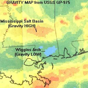 In the Gulf Coast of southernmost Alabama and Mississippi, a barely-visible yellow-green area marks the Wiggins Arch (see enlargement at left). This is a gravity low over a high-standing basement terrane, and the Mississippi Salt Basin, to the north, is a gravity high. One explanation for this unexpected situation is to infer that the Wiggins Arch is a block of relatively low-density crust, left behind as Yucatan rotated away to open the Gulf of Mexico. The Mississippi Salt Basin would be an area of thinned crust, with a high-standing area of relatively dense lower crust or mantle beneath the basin. The crust-mantle density contrast (probably 2.9 to 3.3 vs. 2.67 for crust) is far more important than the relatively thin low-density sediments in the basin (including salt). It is very important in looking at regional gravity data to consider the possibility of crust-mantle effects.
The Llano Uplift, in central Texas, contains outcropping Precambrian rocks. They are overlain on the margins of the uplift by Phanerozoic sedimentary rocks, and the center of the gravity high coincides with the Precambrian outcrop.
The Idaho and Sierra Nevada Batholiths are large gravity lows, indicating that they contain a deep "root" of relatively low-density granitic material, which sticks down into the denser lower crust-upper mantle. Both are much more complicated than that in detail; for example the east side of the Sierra Nevada uplift is a late Tertiary normal fault with great throw. The central Rocky Mountains of Colorado probably have a similar deep low-density mass, to account for the huge low there.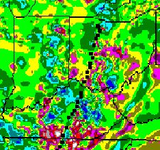 However, some of this effect may be due to other variations in crustal thickness. Also, in the San Juan Mountains (SW Colorado), a large part of the gravity low coincides with a huge pile of Tertiary volcanics. They may have depressed the crust, and their relative low density also may contribute to that part of the regional gravity low.
The Grenville Front, along a NNE-SSW line in Ohio and Kentucky, is a 1-billion-year-old collisional contact between two different terranes. Their differences have some expression in the gravity map, but the front is much more distinctive in a magnetic map, as shown by the black dotted line in the magnetic map on the right. (See also, for example, Gibson's Interpreted Magnetic Basement Terrane Map of the U.S.)
Disagreements? Let me know! . Below is a magnetic map of the US (from USGS).
©2000-2010 Richard I. Gibson
Richard I. Gibson,
Gibson Consulting -
301 North Crystal St. -
Butte, Montana 59701 -
Phone: 406-490-1556 - E-mail